写在博客之前

数据预处理

处理非数值型数据

import pandas as pd  

df = pd.DataFrame([ 
                    ['green', 'M', 10.1, 'class1'], 
                    ['red', 'L', 13.5, 'class2'], 
                    ['blue', 'XL', 15.3, 'class1']]) 
df.columns = ['color', 'size', 'price', 'classlabel'] 
print(df)

   color size  price classlabel
0  green    M   10.1     class1
1    red    L   13.5     class2
2   blue   XL   15.3     class1

利用pandas将CSV格式的数据读取进来，要将字符串转换为适合机器学习算法训练的数据类型。
先对特征size数据进行处理，由于XL>L>M，size特征有这样的一个顺序特征，所以将这类字符串转换为数值时也该保留顺序特征。利用映射函数map很容易将字符串转换：

size_mapping = {                  
                'XL': 3,                  
                'L': 2,                
                'M': 1} 
df['size'] = df['size'].map(size_mapping) 
print(df)

   color  size  price classlabel
0  green     1   10.1     class1
1    red     2   13.5     class2
2   blue     3   15.3     class1

可以利用小技巧将数值数据转换回字符串：

inv_size_mapping = {v: k for k, v in size_mapping.items()}
print(df['size'].map(inv_size_mapping) )

0     M
1     L
2    XL
Name: size, dtype: object

对于分类标签classlabe，只需要将字符串转换为数值特征就好。
利用枚举函数enumerate()和np.unique()将标签导出为映射字典，在用映射函数map将分类标签转换为整数：

import numpy as np
class_mapping = {label:idx for idx,label in                 
                 enumerate(np.unique(df['classlabel']))}
df['classlabel'] = df['classlabel'].map(class_mapping) 
print(df)

   color  size  price  classlabel
0  green     1   10.1           0
1    red     2   13.5           1
2   blue     3   15.3           0

同样将整数值可以反映射回分类标签：

inv_class_mapping = {v: k for k, v in class_mapping.items()}
df['classlabel'] = df['classlabel'].map(inv_class_mapping) 
print(df)

   color  size  price classlabel
0  green     1   10.1     class1
1    red     2   13.5     class2
2   blue     3   15.3     class1

也可直接调用sklearn库LabelEncoder类实现：

from sklearn.preprocessing import LabelEncoder 

class_le = LabelEncoder() 
y = class_le.fit_transform(df['classlabel'].values) 
print(y)

[0 1 0]

class_le.inverse_transform(y)

array(['class1', 'class2', 'class1'], dtype=object)

接下来考虑特征color，颜色green，red，blue没有顺序特征，可以采用热编码的方式将其转换，调用pandas中的get_dummies方法转换字符串：

pd.get_dummies(df[['price', 'color', 'size']])

	price	size	color_blue	color_green	color_red
0	10.1	1	0	1	0
1	13.5	2	0	0	1
2	15.3	3	1	0	0

划分数据集为训练集和测试集

import pandas as pd
import numpy as np

df_wine = pd.read_csv('https://archive.ics.uci.edu/'                          
                       'ml/machine-learning-databases/'                          
                       'wine/wine.data', header=None) 
df_wine.columns = ['Class label', 'Alcohol',                  
                       'Malic acid', 'Ash',                
                       'Alcalinity of ash', 'Magnesium',                 
                       'Total phenols', 'Flavanoids',                    
                       'Nonflavanoid phenols',                    
                       'Proanthocyanins',                     
                       'Color intensity', 'Hue',                     
                       'OD280/OD315 of diluted wines',                     
                       'Proline']  
print('Class labels', np.unique(df_wine['Class label'])) 
df_wine.head()

Class labels [1 2 3]

	Class label	Alcohol	Malic acid	Ash	Alcalinity of ash	Magnesium	Total phenols	Flavanoids	Nonflavanoid phenols	Proanthocyanins	Color intensity	Hue	OD280/OD315 of diluted wines	Proline
0	1	14.23	1.71	2.43	15.6	127	2.80	3.06	0.28	2.29	5.64	1.04	3.92	1065
1	1	13.20	1.78	2.14	11.2	100	2.65	2.76	0.26	1.28	4.38	1.05	3.40	1050
2	1	13.16	2.36	2.67	18.6	101	2.80	3.24	0.30	2.81	5.68	1.03	3.17	1185
3	1	14.37	1.95	2.50	16.8	113	3.85	3.49	0.24	2.18	7.80	0.86	3.45	1480
4	1	13.24	2.59	2.87	21.0	118	2.80	2.69	0.39	1.82	4.32	1.04	2.93	735

首先将数据读取，调用train_test_split函数将数据集划分，参数test_size=0.3表示将数据集的30%
划分给测试集，把70%划分给训练集，stratify=y表示训练集中各个类别的比例和测试集中一样。

from sklearn.model_selection import train_test_split 

X, y = df_wine.iloc[:, 1:].values, df_wine.iloc[:, 0].values 
X_train, X_test, y_train, y_test =train_test_split(X, y,                      
                                             test_size=0.3,                      
                                             random_state=0,                     
                                             stratify=y)

数据正则化

数据正则化对线性模型和梯度下降等优化算法特别有用。但基于树的模型不需要进行标准化。
创建StandardScaler对象，调用fit方法获取样本均值和标准差，再用这些参数去转换测试集。

from sklearn.preprocessing import StandardScaler 

sc = StandardScaler() 
sc.fit(X_train) 
X_train_std = sc.transform(X_train)
X_test_std = sc.transform(X_test) 

特征的选择

L1正则化：

import matplotlib.pyplot as plt
from sklearn.linear_model import LogisticRegression

fig = plt.figure() 
ax = plt.subplot(111)
colors = ['blue', 'green', 'red', 'cyan', 
          'magenta', 'yellow', 'black', 
          'pink', 'lightgreen', 'lightblue', 
          'gray', 'indigo', 'orange'] 
weights, params = [], []
for c in np.arange(-4., 6.): 
    lr = LogisticRegression(penalty='l1', 
                            C=10.**c, 
                            random_state=0,solver='liblinear',multi_class='ovr') 
    lr.fit(X_train_std, y_train)
    weights.append(lr.coef_[1])
    params.append(10**c)
weights = np.array(weights)
for column, color in zip(range(weights.shape[1]), colors):
    plt.plot(params, weights[:, column],
             label=df_wine.columns[column + 1],
             color=color) 
plt.axhline(0, color='black', linestyle='--', linewidth=3)
plt.xlim([10**(-5), 10**5])
plt.ylabel('weight coefficient')
plt.xlabel('C') 
plt.xscale('log')
plt.legend(loc='upper left')
ax.legend(loc='upper center',
          bbox_to_anchor=(1.38, 1.03),
          ncol=1, fancybox=True)
plt.show()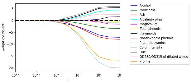 

纵轴对应各个特征的权重，横轴参数C是正则化参数的逆，参数C越小，模型的正则化强度就越强，上述采用L1正则化，可以看到，当C极小的时候，各个特征的权值都趋近于0，然而，当C越大时，有些特征的权重依然徘徊在0附近，这说明对于该分类模型来说，这些特征对于分类的作用没有那么明显，所以，我们可以在训练模型的时候将这些模型去掉，以简化分类模型，减少泛化误差。可以说，L1正则化是一种特征选择技术。

---

转载请注明来源，欢迎对文章中的引用来源进行考证，欢迎指出任何有错误或不够清晰的表达。可以在下面评论区评论，也可以邮件至 572108581@qq.com